Linear Programming | ||
| ||
Introduction | ||
In this section, you will learn about linear programming. Here are the sections within this lesson:
|
Linear programming is the name for a logistic process that maximizes effort. It is a practical application for maximizing profit for businesses, which is the context for the lessons that will follow. However, let it be known that linear programming was invented by mathematically-minded thinkers for war. In order to determine the best way to move supplies (like gasoline, food, soldiers, …) to place them where they were immediately needed to increase the effectiveness for military campaigns, this mathematics was developed. It turned out that this mathematics had broader applications than war alone. So, students learn it to make important changes to businesses to increase their potential and make greater profit.
Linear Programming can also be applied to strategy games, much like Clash of Clans, to optimize performance and be a better player.
| |
To do linear programming problems, we have to know a lot of mathematics. MATHguide already has lessons on these and please review them as needed throughout this lesson on linear programming.
| |
Businesses have certain limitations. They can have only so many workers do to the size of their facilities. Businesses can only hold so many items on a truck. They can afford to have only so many trucks. Businesses only have so much revenue to work with and have to operate within that budget. Keeping these limitations in mind, we will now look at statements and convert them into inequalities. Example 1: “Jim has to move at least 20 cattle each day.” Jim’s job obviously depends on cattle. Let ‘x’ stand for the number of cattle he moves each day. He cannot move less than 20 cattle; so, he must move more than 20. This is best represented using a greater than sign.

This answer is correct only because we designated that the ‘x’ stands for the number of cattle. It was a crucial step that cannot be ignored.
Example 2: “Julio cannot sell more than 30 burritos and no more than 50 tacos, due to the small size of his food truck.” There are two quantities being discussed here: burritos and tacos. Let ‘x’ stand for the number of burritos and let ‘y’ stand for the number of tacos. He cannot sell more than the 30 and the 50, respectively. So, he must sell less than those amounts. We will use less than signs for each inequality.
 ideo: Linear Programming: Constructing Inequalities ideo: Linear Programming: Constructing Inequalities
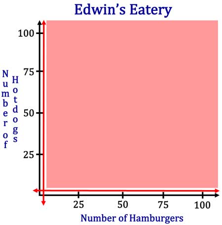
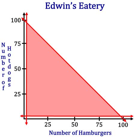
Example 3: “Edwin is selling hamburgers and hotdogs from his small stand in a mall. He has to sell at least 5 hamburgers and at least 4 hotdogs each day to break even. He cannot sell more than a total of 100 food items.” Let ‘x’ stand for the number of hamburgers and let ‘y’ stand for the number of hotdogs. There are three inequalities for this problem. Let’s take a look at them, one at a time:
| |
The objective function is the function we use to determine maximum or minimum values. As it applies to business models, we call them profit functions. We will look at two examples to get profit functions. Example 1: “Maria, an employee at Burger Barn, charges her customer $2.50 for hamburgers and $1.50 for fries.” First, we have to set up the variables, which is an important step. Let ‘x’ stand for the number of hamburgers and let ‘y’ stand for the number of fries. This would be the profit function.
The function is written as P(x,y) because the function requires to values. It requires an ‘x’ and a ‘y.’ If Maria sells 20 hamburgers and 10 fries during lunch, we can calculate the profit for lunch, as follows.
Example 2: “Pete sells furniture. He charges $200 for tables and $75 for chairs.” We will start by setting up the variables. Let ‘x’ stand for the number of tables and let ‘y’ stand for the number of chairs. This would be the profit function.
If Pete sells 30 tables and 150 chairs in a month, we can calculate the profit, as follows.
| |
The feasible region is defined as the mathematical operating space for a business. If a business’ limitations allow for it, a unique region will result from the inequalities we graph. This means we will have to know how to graph lines and inequalities. Please review the graphing lessons if you either do not know how to graph lines or if the following material becomes confusing to you. If we look at Example 3 from the Section: Converting Words into Symbols, notice that we had this system of inequalities for the answer. Here is that system, but the inequalities have been numbered for reference.
The first inequality is a vertical line and it’s shaded to the right. The second inequality is a horizontal line and it’s shaded above. This is what the graph looks like, so far.
The third inequality is a diagonal line. Once we temporarily think of the diagonal line as an equation, will use our knowledge of Graphing Lines in Standard Form. After testing (0,0), which works and it’s below the line, we can see that we shade below the line. Our new graph now looks like this.
The next section will take this problem one step farther. We will look at finding the vertices of this feasible region. | |
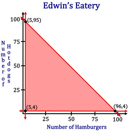
Let’s continue to look at the last problem. Here is the graph we obtained but the vertices (or points of intersection) have been lettered for reference.

Now, we will locate each of the three vertices. Point A: This point is the intersection of the vertical and horizontal lines. It’s the easiest to find because we know the x-value is 5 and the y-value is 4. Therefore, the point is (5,4) Point B: This is the point where the vertical line intersects the diagonal line. To locate this point takes a little bit of work. We will take the diagonal line without the inequality and substitute the x-value of 5. Then, we will solve for y, like so.
This means the point is at (5,95). Point C: This is the location where the horizontal line intersects the diagonal line. This point has a y-value of 4. We will substitute this value into the diagonal line and solve for the x-value.
This means the point is at (95,4). Here is the region with the vertices.
| |
For our last problem, we concluded with a graph of the feasible region and we located the vertices of the feasible region. Now, we are going to evaluate the vertices within a profit function. MATHguide has a lesson on Evaluating (Single Variable) Functions, which means substituting for x-values only. However, these linear programming problems require substituting two values at a time, a x-value and a y-value. If the hamburgers go for $3.00 and the hotdogs go for $2.00, this is our objective equation.
We will now evaluate each of the vertices within this profit function.
We can see that P(96,4) gives us a maximum of 296. | |
We are going to take a look at a complete problem, from beginning to end. However, the steps will be slightly abbreviated. If you find any of the steps to be confusing, either review MATHguide’s related lessons or look at the examples above. Here is a problem.
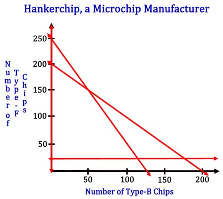
“Hank makes two popular types of microchips for computers, type B18 and type F91. One of his customers needs at least 20 type-F chips per day. He cannot produce more than 200 microchips per day. Due to his supplier, the sum of twice the type-B chips and type-F chips cannot be more than 250. How many chips of each type must he sell to maximize his profit if he sells the type-B chips at $15 and type-F chips at $18?” We need to take the problem, line by line to get the inequalities. We also need to declare that the x-value stands for type-B chips and the y-value stands for type-F chips.
The implied inequality is present even though it has not been specifically mentioned in the problem. The reason it is there is because it is impossible to produce a negative number of chips. Now, we are going to graph these inequalities on a coordinate plane. Here they are before being shaded.
Here, the feasible region is now shown.
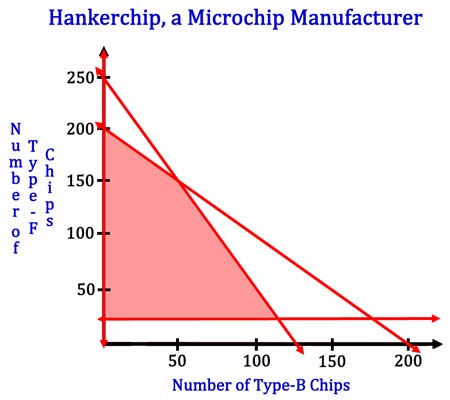
Next, we will locate the vertices of the feasible region. You may need to look over our section on Systems of Equations to understand how to locate points of intersection. Nevertheless, here are those vertices.
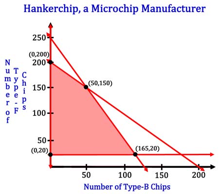
Now we will evaluate the profit function at each vertex with this profit function.
It is clear that the maximum value is from P(0,200), which is 3600. Since the x-values stand for type-B chips, it is evident that Hank needs to stop selling type-B chips and he needs to sell 200 type-F chips per day to maximize profits.
| |
Try our instructional videos to help you learn.
| |
Try our interactive quizzes to determine if you understand the lessons above.
| |
Try this activity related to the lessons above.
| |
Try these lessons, which are related to the lesson above.
| |
 esson:

 uizmaster:
  ctivity: